Examples
The following sections contain some usage examples of CellSium.
Creating random training data
The core mode of operation is the creation of ground truth data as training data for machine learning/deep learning applications. To this end, CellSium contains two output modes specifically tailored to produce outputs for common deep learning based object detectors/instance segmentation toolkits: The COCO and YOLO format. CellSium can as well just output binary masks along the images for use with other learning tools.
For example, the following command will random cell images, and output three datasets:
> python -m cellsium training \
    -t TrainingDataCount=64 \
    -t TrainingCellCount=512 \
    -t TrainingImageWidth=512 \
    -t TrainingImageHeight=512 \
    -t Calibration=0.0905158 \
    -t ChipmunkPlacementRadius=0.01 \
    -o training \
    --Output COCOOutput \
    --Output YOLOOutput \
    --Output GenericMaskOutput \
    -p
Note how the main mode of configuration of CellSium are tunables, these tunable parameters are set using the -t argument, followed by Name=value. The tunables are explained in the documentation, and can be listed via --tunables-show as well.
In this example, the output of 64 images of 512x512 size are requested, setting the pixel calibration to 0.0905158 µm per pixel. ChipmunkPlacementRadius configures the physical placement and yields denser colonies. The name of the output files/directories is specified using -o.
The outputs of CellSium are modular. In this example, the COCOOutput, YOLOOutput, and GenericMaskOutput are enabled. As to prevent name clashes and allow easy coexistence, the -p:code: switch enables prefixing of the output names with the name of the respective output module.
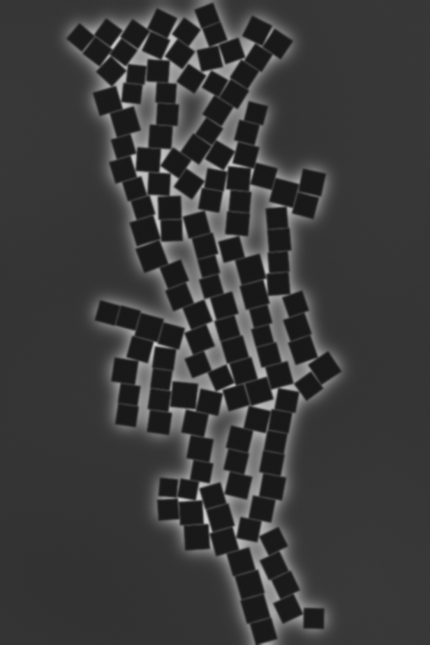
Once the exmaple has run, the directories COCOOutput-training, GenericMaskOutput-training, and YOLOOutput-training have been created, with examples of the GenericMaskOutput shown.
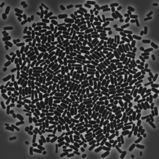
|
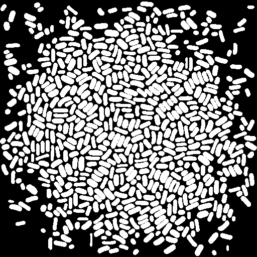
|
Creating a timelapse simulation
CellSium was originally developed to create time lapse simulations to create realistic microcolonies, which can serve as input data e.g., for simulations based on the geometry or the training and validation of tracking algorithms.
To run a simulation, ste up the desired outputs and tunables as explained, and use the simulate subcommand.
> python -m cellsium simulate \
    -o simulate \
    --Output GenericMaskOutput \
    --Output TiffOutput \
    -p
In this case, a microcolony will be simulated, a time lapse TIFF stack as well as mask output generated. Shown are three example images:
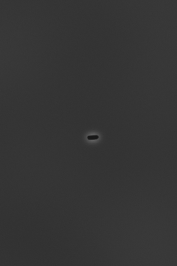
|

|
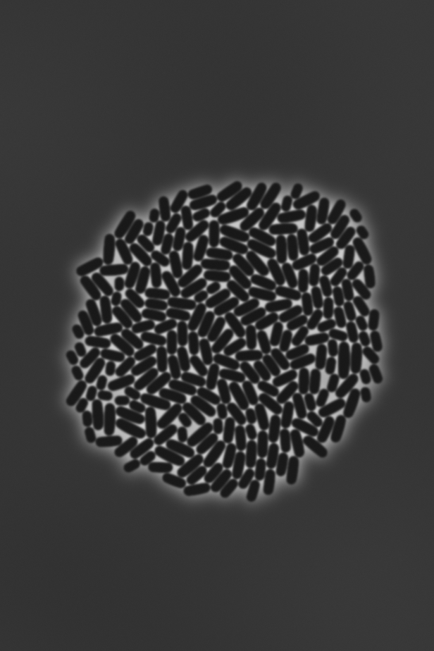
|
Adding a custom cell model
In the previous examples, the standard (sizer) cell model was used. However, the modular nature of CellSium makes it easy to integrate a custom cell model. In this example, the sizer model will be defined externally, so it can be more easily changed, and to showcase its difference, the easter egg square geometry will be applied:
from cellsium.model import assemble_cell, SimulatedCell, h_to_s, Square


class SquareCellModel(SimulatedCell):
    @staticmethod
    def random_sequences(sequence):
        return dict(elongation_rate=sequence.normal(1.5, 0.25))  # µm·h⁻¹

    def birth(self, parent=None, ts=None) -> None:
        self.elongation_rate = next(self.random.elongation_rate)
        self.division_time = h_to_s(1.0)

    def grow(self, ts) -> None:
        self.length += self.elongation_rate * ts.hours

        if ts.time > (self.birth_time + self.division_time):
            offspring_a, offspring_b = self.divide(ts)
            offspring_a.length = offspring_b.length = self.length / 2


Cell = assemble_cell(SquareCellModel, Square)
The custom model can be specified using the -c switch, specifying either an importable Python module, or the path of a Python file. If no class name is specified after the : colon, CellSium will attempt to import a class named Cell from the file/module.
> python -m cellsium simulate \
    -o square \
    --Output GenericMaskOutput \
    -c square.py:Cell \
    -p
CellSium cell objects are Python objects. They are built lending from OOP principles, using mixins in a very flexible way to join various properties. To gain deeper insights how to implement and alter cellular behavior or rendering, it is best to study the source code of CellSium.
|
Jupyter Notebook Embedding Example
In this example, CellSium is embedded in a Jupyter notebook to interactively run small simulations.
First, the necessary modules are imported:
# plotting
from matplotlib_inline.backend_inline import set_matplotlib_formats
set_matplotlib_formats('svg')
from matplotlib import pyplot

# general
from functools import partial

# RRF is the central random helper, used for seeding
from cellsium.random import RRF
# the model parts the new model is built upon
from cellsium.model import PlacedCell, SimulatedCell, assemble_cell
# the functions to actually perform the simulation
from cellsium.cli.simulate import perform_simulation, initialize_cells, h_to_s, s_to_h
# the PlotRenderer as it embeds nicely in Jupyter
from cellsium.output.plot import PlotRenderer
For the example, a model is defined directly within a Jupyter cell:
class SizerCell(SimulatedCell):
    @staticmethod
    def random_sequences(sequence):
        return dict(elongation_rate=sequence.normal(1.5, 0.25))  # µm·h⁻¹

    def birth(
        self, parent=None, ts=None
    ) -> None:
        self.elongation_rate = next(self.random.elongation_rate)
        self.division_time = h_to_s(0.5)  # fast division rate

    def grow(self, ts):
        self.length += self.elongation_rate * ts.hours

        if ts.time > (self.birth_time + self.division_time):
            offspring_a, offspring_b = self.divide(ts)
            offspring_a.length = offspring_b.length = self.length / 2
# seed the random number generator
RRF.seed(1)

# perform_simulation returns an iterator which will indefinitely yield timesteps

simulation_iterator = perform_simulation(
    setup=partial(
        initialize_cells,
        count=1,
        cell_type=assemble_cell(SizerCell, placed_cell=PlacedCell)),
    time_step=30.0 * 60.0
)

# we step thru the first 5 of them ...
for _, ts in zip(range(5), simulation_iterator):
    # ... and plot them
    PlotRenderer().output(world=ts.world)
    pyplot.title("Simulation output at time=%.2fh" % (s_to_h(ts.time)))
    pyplot.show()
    # we have access to the Cell objects as well
    print(repr(ts.world.cells))

[Cell(angle=2.3294692309443428, bend_lower=-0.016261360844027475, bend_overall=-0.04126808565523994, bend_upper=-0.09614075306364522, birth_time=0.0, division_time=1800.0, elongation_rate=1.5981931788501658, id_=1, length=2.872894940610261, lineage_history=[0], parent_id=0, position=[17.854225629902448, 28.67645476278087], width=0.8960666826747447)]

[Cell(angle=2.3294692309443428, bend_lower=-0.016261360844027475, bend_overall=-0.04126808565523994, bend_upper=-0.09614075306364522, birth_time=3600.0, division_time=1800.0, elongation_rate=1.4017119040732795, id_=2, length=1.835995765017672, lineage_history=[0, 1], parent_id=1, position=[18.485770454254308, 28.010218132802386], width=0.8960666826747447), Cell(angle=2.3294692309443428, bend_lower=-0.016261360844027475, bend_overall=-0.04126808565523994, bend_upper=-0.09614075306364522, birth_time=3600.0, division_time=1800.0, elongation_rate=1.7743185975635118, id_=3, length=1.835995765017672, lineage_history=[0, 1], parent_id=1, position=[17.22268080555059, 29.342691392759356], width=0.8960666826747447)]

[Cell(angle=2.3360626329715437, bend_lower=-0.016261360844027475, bend_overall=-0.04126808565523994, bend_upper=-0.09614075306364522, birth_time=3600.0, division_time=1800.0, elongation_rate=1.4017119040732795, id_=2, length=2.5368517170543115, lineage_history=[0, 1], parent_id=1, position=[18.756872759489948, 27.72423023484169], width=0.8960666826747447), Cell(angle=2.3228640880321927, bend_lower=-0.016261360844027475, bend_overall=-0.04126808565523994, bend_upper=-0.09614075306364522, birth_time=3600.0, division_time=1800.0, elongation_rate=1.7743185975635118, id_=3, length=2.7231550637994277, lineage_history=[0, 1], parent_id=1, position=[16.951578500314948, 29.62867929072005], width=0.8960666826747447)]

[Cell(angle=2.352798559960036, bend_lower=-0.016261360844027475, bend_overall=-0.04126808565523994, bend_upper=-0.09614075306364522, birth_time=7200.0, division_time=1800.0, elongation_rate=0.8317980611709823, id_=4, length=1.6188538345454755, lineage_history=[0, 1, 2], parent_id=2, position=[19.593155424028517, 26.85358455987381], width=0.8960666826747447), Cell(angle=2.3416190585127383, bend_lower=-0.016261360844027475, bend_overall=-0.04126808565523994, bend_upper=-0.09614075306364522, birth_time=7200.0, division_time=1800.0, elongation_rate=1.2231841085165691, id_=5, length=1.6188538345454755, lineage_history=[0, 1, 2], parent_id=2, position=[18.471310193545275, 28.02153383690875], width=0.8960666826747447), Cell(angle=2.314495314084782, bend_lower=-0.016261360844027475, bend_overall=-0.04126808565523994, bend_upper=-0.09614075306364522, birth_time=7200.0, division_time=1800.0, elongation_rate=1.4247110511570817, id_=6, length=1.8051571812905918, lineage_history=[0, 1, 3], parent_id=3, position=[17.289158390942983, 29.25243321304336], width=0.8960666826747447), Cell(angle=2.304654468034007, bend_lower=-0.016261360844027475, bend_overall=-0.04126808565523994, bend_upper=-0.09614075306364522, birth_time=7200.0, division_time=1800.0, elongation_rate=1.8079038604401219, id_=7, length=1.8051571812905918, lineage_history=[0, 1, 3], parent_id=3, position=[16.06327851109302, 30.578267441297573], width=0.8960666826747447)]

[Cell(angle=2.3820603181599442, bend_lower=-0.016261360844027475, bend_overall=-0.04126808565523994, bend_upper=-0.09614075306364522, birth_time=7200.0, division_time=1800.0, elongation_rate=0.8317980611709823, id_=4, length=2.0347528651309665, lineage_history=[0, 1, 2], parent_id=2, position=[20.228643748180197, 26.199313752340714], width=0.8960666826747447), Cell(angle=2.3526475982043165, bend_lower=-0.016261360844027475, bend_overall=-0.04126808565523994, bend_upper=-0.09614075306364522, birth_time=7200.0, division_time=1800.0, elongation_rate=1.2231841085165691, id_=5, length=2.23044588880376, lineage_history=[0, 1, 2], parent_id=2, position=[18.75284683312141, 27.731672298371393], width=0.8960666826747447), Cell(angle=2.2968665429831496, bend_lower=-0.016261360844027475, bend_overall=-0.04126808565523994, bend_upper=-0.09614075306364522, birth_time=7200.0, division_time=1800.0, elongation_rate=1.4247110511570817, id_=6, length=2.5175127068691325, lineage_history=[0, 1, 3], parent_id=3, position=[17.088954083136315, 29.417294148769457], width=0.8960666826747447), Cell(angle=2.2660140670444004, bend_lower=-0.016261360844027475, bend_overall=-0.04126808565523994, bend_upper=-0.09614075306364522, birth_time=7200.0, division_time=1800.0, elongation_rate=1.8079038604401219, id_=7, length=2.709109111510653, lineage_history=[0, 1, 3], parent_id=3, position=[15.346457855171874, 31.35753885164192], width=0.8960666826747447)]